
Three matching sales can show that transactions happened at three recorded prices. They cannot establish a dependable price for every copy of a skin. The useful next step is to test how much the conclusion depends on each observation, then explain what the sample leaves unknown.
A small dataset is still worth reading. You can inspect every row, identify differences and avoid hiding uncertainty behind a precise average. The mistake is asking it to answer more than its size and coverage allow.
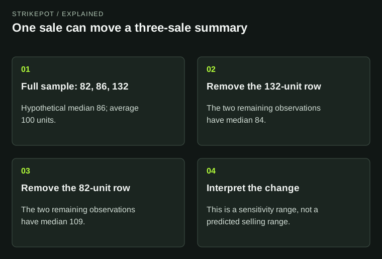
The same tiny dataset supports noticeably different summaries when one observation changes. All amounts are hypothetical.
Start with the evidence you actually have
Suppose you find three completed sales for the same named finish and exterior. All figures in this article are hypothetical, expressed in one currency unit, and do not describe a live market. The recorded amounts are 82, 86 and 132. The average is 100, while the median is 86.
Neither calculation is wrong. They describe different features of those three numbers. Calling the item “a 100-unit skin,” however, removes the fact that one comparatively expensive observation contributes 44% of the sample's total value. Calling 86 its certain sale price creates a different unsupported claim.
Official records can offer different levels of detail. Skinport documents grouped sale statistics; DMarket's 2019 Sales History announcement describes individual recent deals. Use the actual fields available, rather than inventing the individual transactions behind an aggregate.
Remove one row at a time
A simple sensitivity check asks what the summary would become if one observation were unavailable. This is an analytical exercise, not permission to delete inconvenient sales. For a two-value sample, the median below is the average of its two ordered values.
| Hypothetical set | Average | Median |
|---|---|---|
| 82, 86, 132 | 100 | 86 |
| 86, 132 | 109 | 109 |
| 82, 132 | 107 | 107 |
| 82, 86 | 84 | 84 |
The result is fragile: removing a single observation moves the median from 86 to somewhere between 84 and 109. That range is not a confidence interval, a future price range or a model prediction. It measures the influence of individual rows in this particular invented set.
This matters when two apparent references differ by only a few units. A five-unit gap between platforms is hard to interpret if changing one relevant observation alters your own summary by much more. The sensible response is a narrower claim about the available records.
Relevance matters alongside sample size
Adding 100 poorly matched sales does not necessarily resolve the problem. They may concern another exterior, a special category or a different period. A larger number can make an unsuitable comparison look more authoritative without answering the question about your item.
List the attributes required for a match before examining prices. In CS2 that might include finish, exterior and category, followed by a float range, pattern or attached detail when it matters to the comparison. Keep the original rule rather than broadening it only after seeing a result you dislike. The guide to sale comparables explains that initial matching task.
Three close matches and 40 broad matches can be reported separately. They should not automatically be merged into a 43-sale reference. A useful note might say that only three rows met the narrow specification, while a wider set supplied background context.
Age can be the price of a larger sample
Extending the period may add observations, but it also changes the question. Three sales in a recent interval and 30 across a much longer interval describe different evidence. The older observations are not newly completed transactions merely because you retrieved them today.
Compare the narrow and broad windows without choosing a winner in advance. Record the count, date span and matching rule for each. If the longer window produces a very different summary, examine whether older prices, a changed mix of copies or a few influential rows explain the difference.
Do not fill quiet days with invented transactions. A long flat line produced by carrying forward the last known price is a display convention. It is not a sequence of fresh sales at that amount. Keep the observation's age visible in your notes.
Do not turn a count into a sale-time promise
A count of three sales does not tell you how many suitable listings went unsold, how long they waited or whether the same seller relisted an item. Those missing denominators matter if your real question is how quickly your copy might sell.
Likewise, the sample does not show how many independent buyers considered the item. Counting transactions and counting people are separate tasks. Avoid statements such as “three buyers establish demand” unless the source actually identifies three distinct buyers and that is relevant to the claim.
The records can support a bounded description: three observed completed sales met your stated rule in the selected period. A forecast about the next sale needs additional assumptions that this exercise has not established.
Write the uncertainty into the comparison
A useful report preserves the sample rather than hiding it. State its size, period, currency, matching rule and summary. Add a short sensitivity note: one row materially changes the result, or the results remain close after each removal. Either finding is more informative than another decimal place.
If you have only aggregate fields, say that individual-row sensitivity could not be checked. The sales-statistics guide helps distinguish those fields. Do not reverse-engineer a fictional list of sales from a median and a volume count.
For an actual sale, finish with the current quote for your exact item and its conditions. Historical evidence helps you judge that quote; it does not become the quote itself. A small sample is most useful when the reader can see both what it records and where its answer stops.